BACK
Universal Gravitational Constant
EQUIPMENT
|
1 |
Gravitational
Torsion Balance |
AP-8215 |
|
1 |
X-Y
Adjustable Diode Laser |
OS-8526A |
|
1 |
45
cm Steel Rod |
ME-8736 |
|
1 |
Large
Table Clamp |
ME-9472 |
|
1 |
Meter
Stick |
SE-7333 |
INTRODUCTION
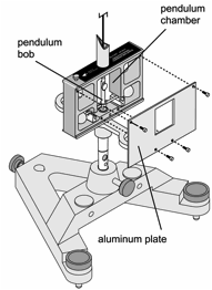
The Gravitational
Torsion Balance reprises one of the great experiments in the history of
physics—the measurement of the gravitational constant, as performed by
Henry Cavendish in 1798.
The Gravitational
Torsion Balance consists of two 38.3 gram masses suspended from a highly
sensitive torsion ribbon and two1.5 kilogram masses that can be positioned as
required. The Gravitational Torsion Balance is oriented so the force of gravity
between the small balls and the earth is negated (the pendulum is nearly
perfectly aligned vertically and horizontally). The large masses are brought
near the smaller masses, and the gravitational force between the large and
small masses is measured by observing the twist of the torsion ribbon.
An optical lever,
produced by a laser light source and a mirror affixed to the torsion pendulum,
is used to accurately measure the small twist of the ribbon.
THEORY
The gravitational
attraction of all objects toward the Earth is obvious. The gravitational
attraction of every object to every other object, however, is anything but
obvious. Despite the lack of direct evidence for any such attraction between
everyday objects, Isaac Newton was able to deduce his law of universal
gravitation.
Newton’s
law of universal gravitation:
![]()
where
m1 and m2 are the masses of the
objects, r is the distance between
them, and
G =
6.67 x 10⁻¹¹ Nm2/kg2
However, in Newton's
time, every measurable example of this gravitational force included the Earth
as one of the masses. It was therefore impossible to measure the constant, G, without first knowing the mass of the
Earth (or vice versa).
The answer to this
problem came from Henry Cavendish in 1798, when he performed experiments with a
torsion balance, measuring the gravitational attraction between relatively
small objects in the laboratory. The value he determined for G allowed the mass and density of the
Earth to be determined. Cavendish's experiment was so well constructed that it
was a hundred years before more accurate measurements were made.
The gravitational
attraction between a 15 gram mass and a 1.5 kg mass when their centers are
separated by a distance of approximately 46.5 mm (a situation similar to that
of the Gravitational Torsion Balance) is about 7 x 10⁻¹⁰ Newtons. If
this doesn’t seem like a small quantity to measure, consider that the weight of
the small mass is more than two hundred million times this amount.
The enormous strength of
the Earth's attraction for the small masses, in comparison with their
attraction for the large masses, is what originally made the measurement of the
gravitational constant such a difficult task. The torsion balance (invented by
Charles Coulomb) provides a means of negating the otherwise overwhelming
effects of the Earth's attraction in this experiment. It also provides a force
delicate enough to counterbalance the tiny gravitational force that exists
between the large and small masses. This force is provided by twisting a very
thin beryllium copper ribbon.

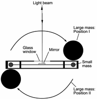
Figure 1: Top View
The large masses are
first arranged in Position I, as shown in Figure 1, and the balance is allowed
to come to equilibrium. The swivel support that holds the large masses is then
rotated, so the large masses are moved to Position II, forcing the system into
disequilibrium. The resulting oscillatory rotation of the system is then
observed by watching the movement of the light spot on the scale, as the light
beam is deflected by the mirror.
SET UP
 Preliminary Set Up
1. Place the support base on a flat, stable table
that is located such that the Gravitational Torsion Balance will be at least 5
meters away from a wall or screen. For best results, use a very sturdy
table, such as an optics table.
2. Carefully secure the Gravitational Torsion
Balance in the base.
3. Remove the front plate by removing the
thumbscrews.
4. Fasten the clear plastic plate to the case with
the thumbscrews.
Figure 2: Removing a plate from the Chamber Box
Leveling the Gravitational Torsion Balance
1. Release the pendulum from the locking mechanism by
unscrewing the locking screws on the case, lowering the locking mechanisms to
their lowest positions (Figure 3).
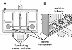
Figure 3: Lowering the Locking Mechanism to
Release the Pendulum Bob Arms
2. Adjust the feet of the base until the pendulum is
centered in the leveling sight (Figure 4). (The base of the pendulum will
appear as a dark circle surrounded by a ring of light).
 3. Orient the
Gravitational Torsion Balance so the mirror on the pendulum bob faces a screen
or wall that is at least 5 meters away.
3. Orient the
Gravitational Torsion Balance so the mirror on the pendulum bob faces a screen
or wall that is at least 5 meters away.
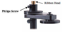

Figure 4: Using the Leveling Sight Figure
5: Adjusting the Height of the Pendulum
Vertical Adjustment of the Pendulum
The base of the pendulum
should be flush with the floor of the pendulum chamber. If it is not, adjust
the height of the pendulum:
1. Grasp the torsion ribbon head and loosen the
Phillips retaining screw (Figure 5a).
2. Adjust the height of the pendulum by moving the
torsion ribbon head up or down so the base of the pendulum is flush with the
floor of the pendulum chamber (Figure 5b).
3. Tighten the retaining (Phillips head) screw.
Rotational Alignment of the Pendulum Bob Arms
(Zeroing)
 The
pendulum bob arms must be centered rotationally in the case — that is,
equidistant from each side of the case (Figure 6). To adjust them:
The
pendulum bob arms must be centered rotationally in the case — that is,
equidistant from each side of the case (Figure 6). To adjust them:
1. Mount a metric scale on the wall or other
projection surface that is at least 5 meters away from the mirror of the
pendulum.
2. Replace the plastic cover with the aluminum
cover.
3. Set up the laser so it will reflect from the mirror
to the projection surface where you will take your measurements (approximately
5 meters from the mirror). You will need to point the laser so that it is
tilted upward toward the mirror and so the reflected beam projects onto the
projection surface (Figure 7). There will also be a fainter beam projected off
the surface of the glass window.
Figure 6: Aligning the Pendulum Bob Rotationally


Figure 7a: Setting
up the Optical Level
(Illustrated
View)
Figure 7b: Setting up the Optical Level
 3. Rotationally align
the case by rotating it until the laser beam projected from the glass window is
centered on the metric scale (Figure 8).
3. Rotationally align
the case by rotating it until the laser beam projected from the glass window is
centered on the metric scale (Figure 8).
Figure 8: Ideal Rotational Alignment
4. Rotationally align the pendulum arm:
a. Raise the locking mechanisms by turning the
locking screws until both of the locking mechanisms barely touch the pendulum
arm. Maintain this position for a few moments until the oscillating energy of
the pendulum is dampened.
b. Carefully lower the locking mechanisms slightly so
the pendulum can swing freely. If necessary, repeat the dampening exercise to
calm any wild oscillations of the pendulum bob.
c. Observe the laser beam reflected from the mirror.
In the optimally aligned system, the equilibrium point of the oscillations of
the beam reflected from the mirror will be vertically aligned below the beam
reflected from the glass surface of the case (Figure 7).

![]()

Figure 9: Refining the Rotational Alignment of
the Pendulum Bob
d. If the spots on the projection surface (the laser
beam reflections) are not aligned vertically, loosen the zero adjust
thumbscrew, turn the zero adjust knob slightly to refine the rotational
alignment of the pendulum bob arms (Figure 9), and wait until the movement of
the pendulum stops or nearly stops.
e. Repeat steps 4a – 4c as necessary until the
spots are aligned vertically on the projection surface.
5. When the rotational alignment is complete,
carefully tighten the zero adjust thumbscrew, being careful to avoid jarring
the system.
Setting up for the Experiment

1. Take an accurate measurement of the distance from the mirror to the zero
point on the scale on the projection surface (L) (Figure 7). (The distance from the mirror surface to the outside
of the glass window is 11.4 mm.)
Note: Avoid jarring the apparatus during this setup
procedure.
Figure 10: Attaching the Grounding Strap to the
Grounding Screw
2. Attach copper wire to the grounding screw (Figure
10), and ground it to the earth.
 3. Place the large
lead masses on the support arm, and rotate the arm to Position I (Figure 11),
taking care to avoid bumping the case with the masses.
3. Place the large
lead masses on the support arm, and rotate the arm to Position I (Figure 11),
taking care to avoid bumping the case with the masses.
4. Allow the pendulum to come to resting
equilibrium.
5. You are now ready to make a measurement using one
of three methods: the final deflection method, the equilibrium method, or the
acceleration method.
Note: The pendulum may require several hours to reach
resting equilibrium. To shorten the time required, dampen the oscillation of
the pendulum by smoothly raising the locking mechanisms up (by turning the
locking screws) until they just touch the crossbar, holding for several seconds
until the oscillations are dampened, and then carefully lowering the locking
mechanisms slightly.
Figure 11: Moving the Large Masses into Position
1
PROCEDURE
1. Once the
steps for leveling, aligning, and setup have been completed (with the large
masses in Position I), allow the pendulum to stop oscillating.
2. Turn on the
laser and observe the Position I end point of the balance for several minutes
to be sure the system is at equilibrium. Record the Position I end point (S1) as accurately as possible, and
indicate any variation over time as part of your margin of error in the
measurement.
3. Carefully
rotate the swivel support so that the large masses are moved to Position II.
The spheres should be just touching the case, but take care to avoid knocking
the case and disturbing the system.
 Note: You can reduce the amount of time the
pendulum requires to move to equilibrium by moving the large masses in a
two-step process: first move the large masses and support to an intermediate
position that is in the midpoint of the total arc (Figure 12), and wait until
the light beam has moved as far as it will go in the period; then move the
sphere across the second half of the arc until the large mass support just
touches the case. Use a slow, smooth motion, and avoid hitting the case when
moving the mass support.
Note: You can reduce the amount of time the
pendulum requires to move to equilibrium by moving the large masses in a
two-step process: first move the large masses and support to an intermediate
position that is in the midpoint of the total arc (Figure 12), and wait until
the light beam has moved as far as it will go in the period; then move the
sphere across the second half of the arc until the large mass support just
touches the case. Use a slow, smooth motion, and avoid hitting the case when
moving the mass support.
4. Immediately after rotating the swivel
support to Position II, observe the light spot. Record the position of the
light spot (S) and the time (t) every 15 seconds. Continue recording
the position and time for about 45 minutes.
5. Rotate the
swivel support to Position I. Repeat the procedure described in step 4.
Note: Although it
is not imperative that step 5 be performed immediately after step 4, it is a
good idea to proceed with it as soon as possible in order to minimize the risk
that the system will be disturbed between the two measurements. Waiting more
than a day to perform step 5 is not advised.
Figure 12: Two-step process of moving the large
masses to reduce the time required to stop oscillating
ANALYSIS
1. Construct a
graph of light spot position versus time for both Position I and Position II.
You will now have a graph similar to Figure 13.

Figure 13: Typical Pendulum Oscillation Pattern
Showing Equilibrium Positions
2. Find the
equilibrium point for each configuration by analyzing the corresponding graphs
using graphical analysis to extrapolate the resting equilibrium points S1 and
S2 (the equilibrium point will be the center line about which the oscillation
occurs). Find the difference between the two equilibrium positions and record
the result as DS.
3. Determine the
period of the oscillations of the small mass system by analyzing the two
graphs. Each graph will produce a slightly different result. Average these
results and record the answer as T.
4. Use your
results and equation 1.9 below to determine the value of G.
Calculating the Value of G
 With the large masses in Position I (Figure
14), the gravitational attraction, F,
between each small mass (m2)
and its neighboring large mass (m1)
is given by the law of universal gravitation:
With the large masses in Position I (Figure
14), the gravitational attraction, F,
between each small mass (m2)
and its neighboring large mass (m1)
is given by the law of universal gravitation:
![]() (1.1)
(1.1)
where b = the distance between the centers of
the two masses.
Figure 14: Origin of Variables b and d
The
gravitational attraction between the two small masses and their neighboring
large masses produces a net torque (tgrav) on the system:
tgrav
= 2Fd
(1.2)
where d is the length of the
lever arm of the pendulum bob crosspiece.
Since the
system is in equilibrium, the twisted torsion band must be supplying an equal
and opposite torque. This torque (tband) is equal to the torsion constant for the
band (k) times the angle through which it is twisted (q), or:
tband
= – kq. (1.3)
Combining
equations 1.1, 1.2, and 1.3, and taking into account that tgrav = – tband, gives:
![]()
Rearranging
this equation gives an expression for G:
![]() (1.4)
(1.4)
To determine
the values of q and k — the
only unknowns in equation 1.4 — it is necessary to observe the
oscillations of the small mass system when the equilibrium is disturbed. To
disturb the equilibrium (from S1), the swivel support is rotated so the large
masses are moved to Position II. The system will then oscillate until it
finally slows down and comes to rest at a new equilibrium position (S2) (Figure
15).

Figure 15: Graph of Small Mass Oscillations
At the new
equilibrium position S2, the torsion
wire will still be twisted through an angle q, but in the
opposite direction of its twist in Position I, so the total change in angle is
equal to 2q.
 Taking into account that the angle is also
doubled upon reflection from the mirror (Figure 16):
Taking into account that the angle is also
doubled upon reflection from the mirror (Figure 16):
![]()
![]() or
or
![]() (1.5)
(1.5)
Figure 16: Diagram of the Experiment Showing the
Optical Level
The torsion
constant can be determined by observing the period (T) of the oscillations, and then using the equation:
![]() (1.6)
(1.6)
where I is the moment of inertia of the small
mass system. The moment of inertia
for the mirror and support system for the small masses is negligibly small
compared to that of the masses themselves, so the total inertia can be
expressed as:
![]()
![]() (1.7)
(1.7)
Therefore:
![]() (1.8)
(1.8)
Substituting
equations 1.5 and 1.8 into equation 1.4 gives:
G=![]() (1.9)
(1.9)
All the
variables on the right side of equation 1.9 are known or
measurable:
r = 9.55 mm
d = 50 mm
b = 46.5 mm
m1
= 1.5 kg
L = (Measure as
in step 1 of the setup.)
By measuring
the total deflection of the light spot (DS) and the period of oscillation (T), the value of G can therefore be determined.
 5.
The value calculated in step 4 is subject to the following systematic
error. The small sphere is attracted not only to its neighboring large sphere,
but also to the more distant large sphere, though with a much smaller force.
The geometry for this second force is shown in Figure 17 (the vector arrows
shown are not proportional to the actual forces).
5.
The value calculated in step 4 is subject to the following systematic
error. The small sphere is attracted not only to its neighboring large sphere,
but also to the more distant large sphere, though with a much smaller force.
The geometry for this second force is shown in Figure 17 (the vector arrows
shown are not proportional to the actual forces).
Figure 17: Correcting the Measured Value of G
From Figure
17,
f=F0sin![]()
![]()
The force, F0
is given by the gravitational law, which translates, in this case, to:
![]()
![]()
and has a
component ƒ that is opposite to the direction of the force F :
![]()
This equation
defines a dimensionless parameter, b,
that is equal to the ratio of the magnitude of ƒ to that of F. Using the equation
![]()
it can be determined that:
![]()
From Figure 17,
![]()
where Fnet is the value of the
force acting on each small sphere from both
large masses, and F is the force
of attraction to the nearest large mass only.
Similarly,
![]()
where G is your experimentally determined
value for the gravitational constant, and G0
is corrected to account for the systematic error.
Finally,
![]()
Use this
equation with equation 1.9 to adjust your measured value.